6  Generalized Autoregressive Conditional Heteroskedasticity (GARCH) Models

The goal of this lecture is to introduce a class of models with conditional heteroskedasticity for stationary time series. You will be able to recognize the presence of such heteroskedasticity from graphs or statistical tests and model it.

Objectives

1. List features of ARCH recognizable from plots.
2. Diagnose ARCH effects using a statistical test.
3. Define ARCH(\(p\)) and GARCH(\(p, q\)) models and identify the orders \(p\) and \(q\).
4. Estimate the models and generate forecasts.
5. Discuss further extensions of the models.

Reading materials

• Chapter 7 in Kirchgässner and Wolters (2007)

6.1 Introduction

In contrast to the traditional time series analysis that focuses on modeling the conditional first moment, models of autoregressive conditional heteroskedasticity (ARCH) and generalized autoregressive conditional heteroskedasticity (GARCH) specifically take the dependency of the conditional second moment into modeling consideration and accommodate the increasingly important need to explain and model risk and uncertainty in, for example, financial time series.

The ARCH models were introduced in 1982 by Robert Engle to model varying (conditional) variance or volatility of time series. It is often found in economics that the larger values of time series also lead to larger instability (i.e., larger variances), which is termed (conditional) heteroskedasticity. Standard examples for demonstrating ARCH or GARCH effects are time series of stock prices, interest and foreign exchange rates, and even some environmental processes: high-frequency data on wind speed, energy production, air quality, etc. (see examples in Cripps and Dunsmuir 2003; Marinova and McAleer 2003; Taylor and Buizza 2004; Campbell and Diebold 2005). In 2003, Robert F. Engle was awarded 1/2 of the Sveriges Riksbank Prize in Economic Sciences in Memory of Alfred Nobel for his work on ARCH models (the other half was awarded to C. Granger, see Section 8.3). Although it is not one of the prizes that Alfred Nobel established in his will in 1895, the Sveriges Riksbank Prize is referred to along with the other Nobel Prizes by the Nobel Foundation.

6.2 Features of ARCH

Since financial data typically have the autocorrelation coefficient close to 1 at lag 1 (e.g., the exchange rate between the US and Canadian dollar hardly changes from today to tomorrow), it is much more interesting and also more practically relevant to model the returns of a financial time series rather than the series itself. Let \(Y_t\) be a time series of stock prices. The returns \(X_t\) measure the relative changes in price and are typically defined as simple returns \[ X_t = \frac{Y_t - Y_{t-1}}{ Y_{t-1} } = \frac{Y_t}{ Y_{t-1} } - 1 \tag{6.1}\] or logarithmic returns \[ X_t = \ln Y_t - \ln Y_{t-1}. \tag{6.2}\] The two forms are approximately the same, since \[ \begin{split} \ln Y_t - \ln Y_{t-1} &= \ln \left(\frac{Y_{t}}{Y_{t-1}} \right) \\ &= \ln \left(\frac{Y_{t-1} + Y_{t} - Y_{t-1}}{Y_{t-1}} \right) \\ &= \ln \left(1 + \frac{Y_{t} - Y_{t-1}}{Y_{t-1}} \right) \\ &\approx \frac{ Y_{t} - Y_{t-1}}{ Y_{t -1} }. \end{split} \tag{6.3}\] The approximation \(\ln(1+x) \approx x\) works when \(x\) is close to zero, which is true for many real-world financial problems. However, logarithmic returns are often preferred because in many applications their distribution is closer to normal compared to one of simple returns. Also, log returns have infinite support (from \(-\infty\) to \(+\infty\)) compared to simple returns that have a lower bound of \(-1\).

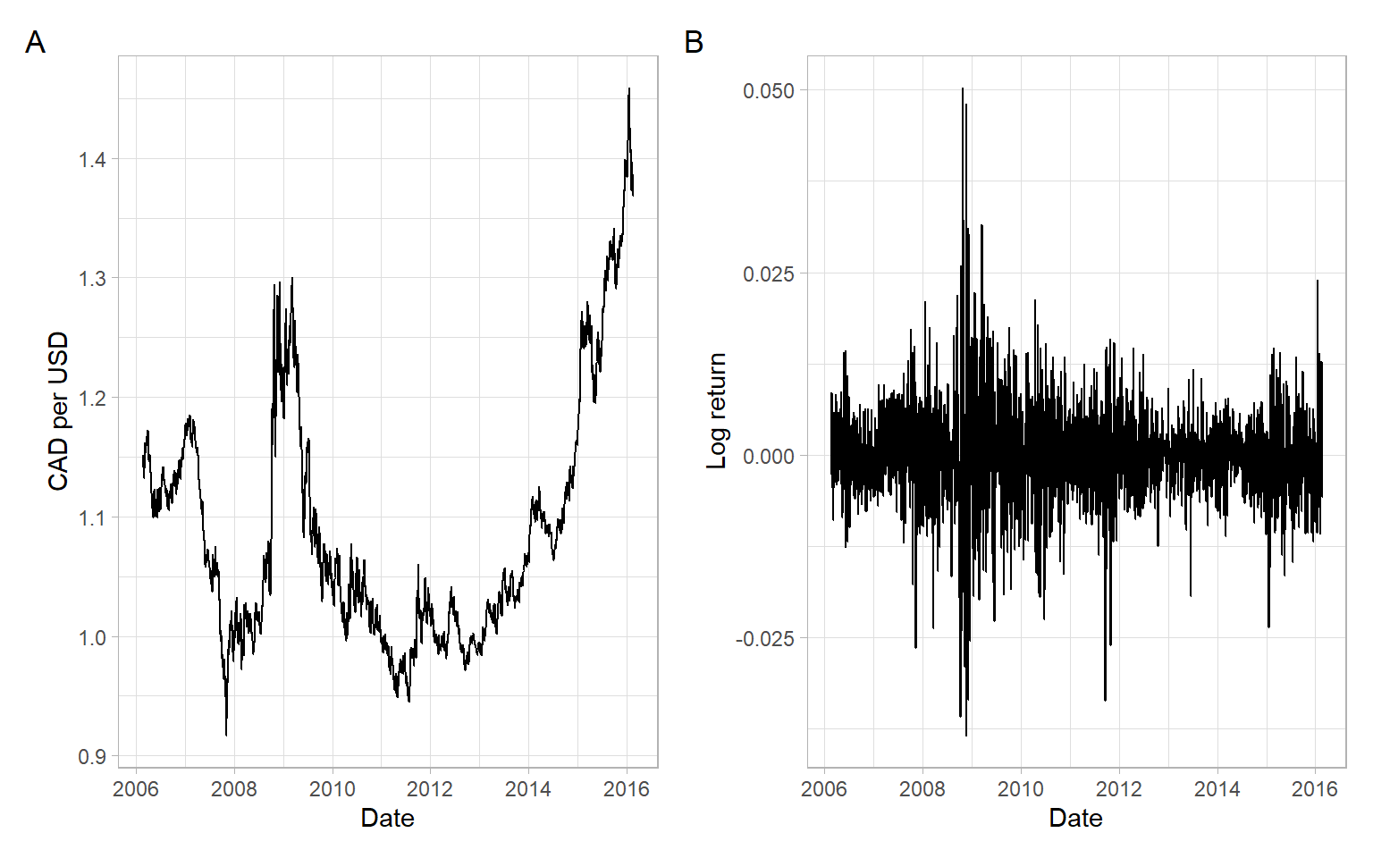
For an example calculation of log returns, see Figure 6.1.

Code

# Load data and calculate log returns
CAD <- readr::read_csv("data/CAD.csv",
                       na = "Bank holiday",
                       skip = 11) %>% 
    filter(!is.na(USD)) %>% 
    mutate(lnR = c(NA, diff(log(USD)))) %>% 
    filter(!is.na(lnR))

p1 <- ggplot(CAD, aes(x = Date, y = USD)) + 
    geom_line() +
    ylab("CAD per USD")
p2 <- ggplot(CAD, aes(x = Date, y = lnR)) + 
    geom_line() +
    ylab("Log return")
p1 + p2 +
    plot_annotation(tag_levels = 'A')

Figure 6.1: CAD per USD daily noon exchange rates and log returns, from 2006-02-22 to 2016-02-22 (excluding bank holidays), obtained from Bank of Canada.

Rydberg (2000) summarizes some important stylized features of financial return series, which have been repeatedly observed in all kinds of assets including stock prices, interest rates, and foreign exchange rates:

1. Heavy tails. The distribution of the returns \(X_t\) has tails heavier than the tails of a normal distribution.
2. Volatility clustering. Large price changes occur in clusters. Indeed, often large price changes tend to be followed by large price changes, and periods of tranquility alternate with periods of high volatility.
3. Asymmetry. There is evidence that the distribution of stock returns is slightly negatively skewed. One possible explanation could be that trades react more strongly to negative information than to positive information.
4. Aggregational Gaussianity. When the sampling frequency decreases, the central limit law sets in and the distribution of the returns over a long period tends toward a normal distribution.
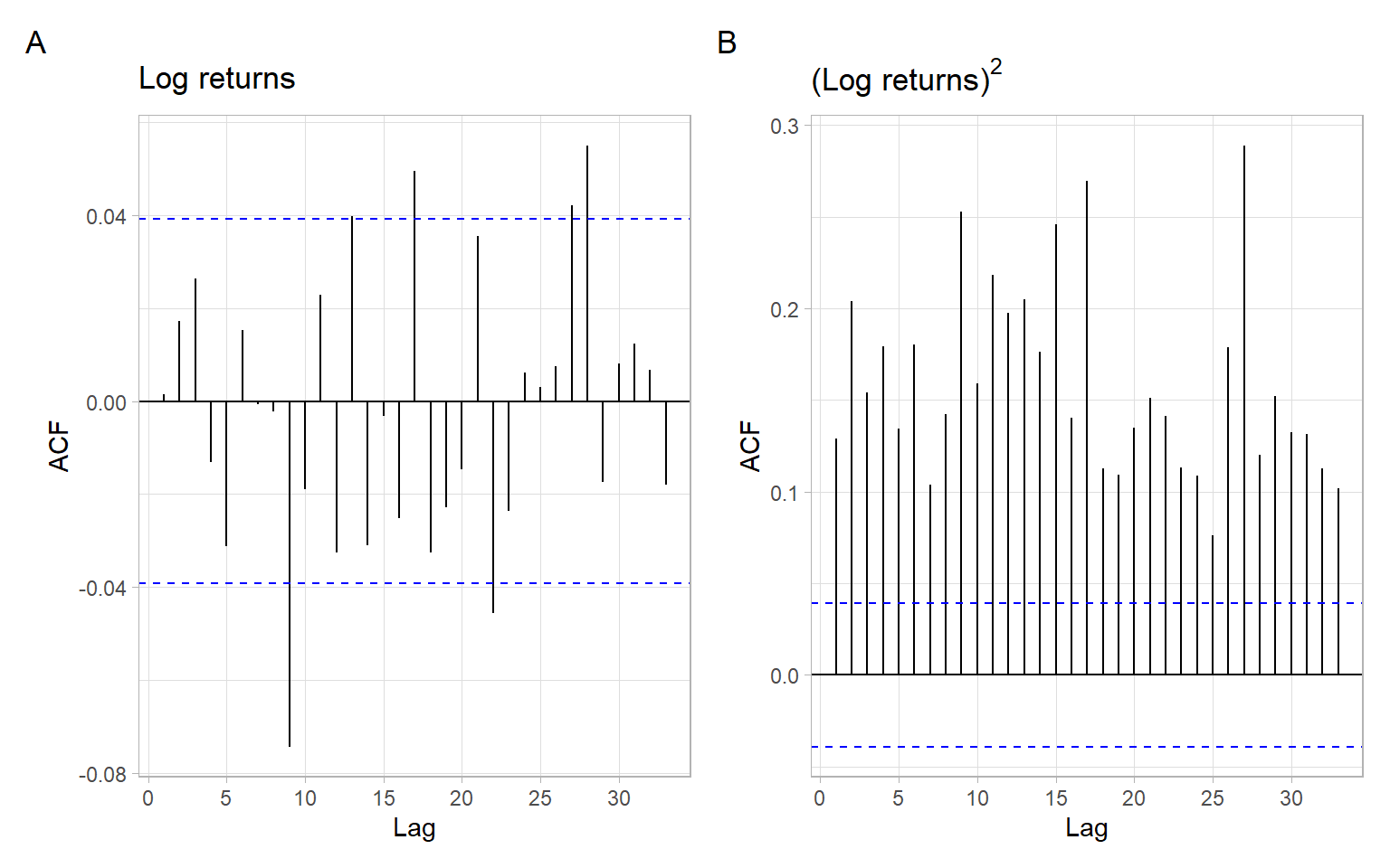
5. Long-range dependence. The returns themselves hardly show any autocorrelation, which, however, does not mean that they are independent. Both squared returns and absolute returns often exhibit persistent autocorrelations indicating possible long-memory dependence in those series.

Figure 6.2 is the simplest check for the presence of ARCH effects: when the time series is not autocorrelated but is autocorrelated if squared.

Code

p1 <- forecast::ggAcf(CAD$lnR) +
    ggtitle("Log returns")
p2 <- forecast::ggAcf(CAD$lnR^2) +
    ggtitle(bquote('(Log returns)'^2))
p1 + p2 +
    plot_annotation(tag_levels = 'A')

Figure 6.2: ACF of log returns and squared log returns for USD/CAD exchange.

For comparison, see Figure 6.3 with similar plots for simulated i.i.d. series.

Code

set.seed(1)
iid <- rnorm(nrow(CAD))

p1 <- forecast::ggAcf(iid) +
    ggtitle("iid")
p2 <- forecast::ggAcf(iid^2) +
    ggtitle(bquote('iid'^2))
p1 + p2 +
    plot_annotation(tag_levels = 'A')

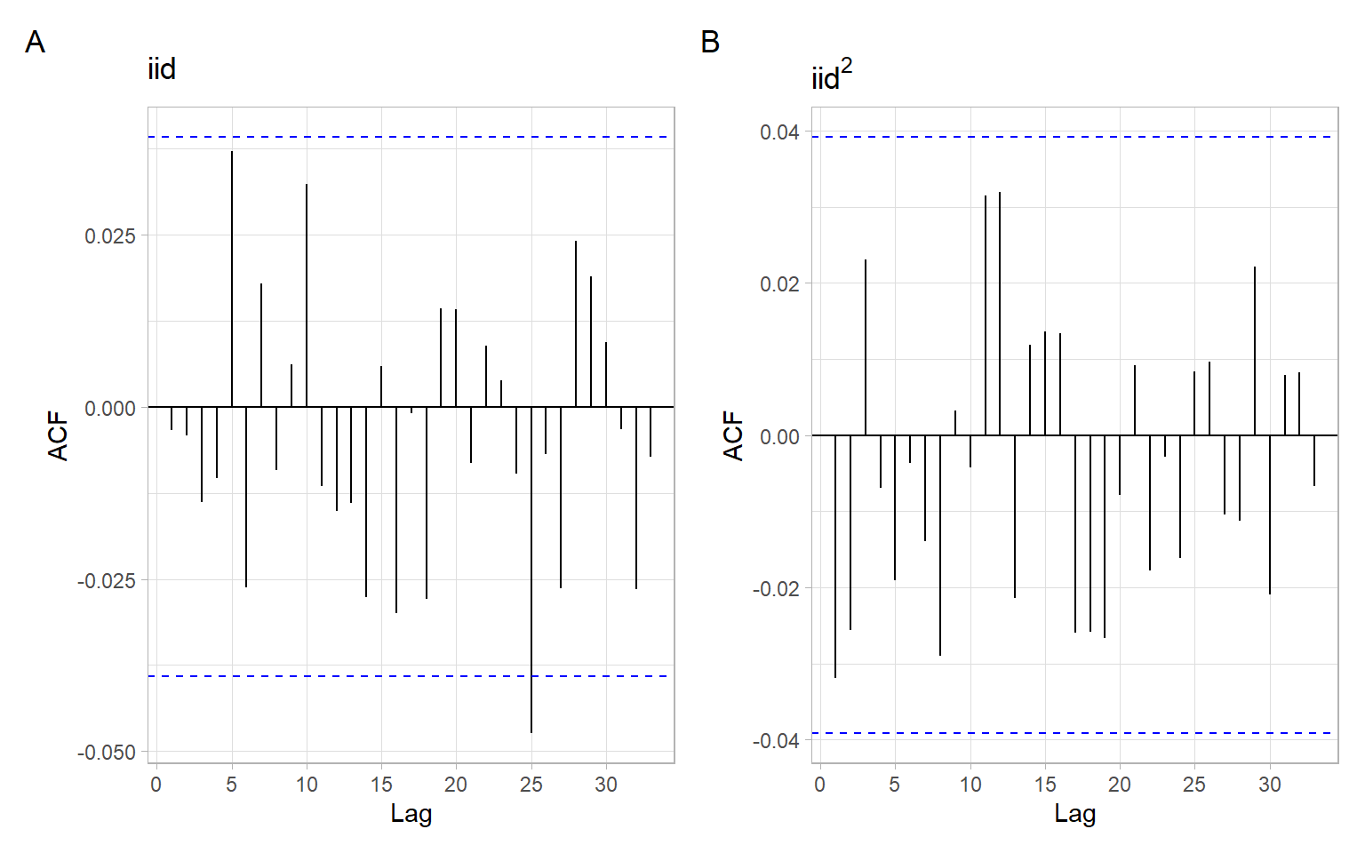
Figure 6.3: ACF of simulated i.i.d. \(N(0,1)\) series.

6.3 Models

Engle (1982) defines an autoregressive conditional heteroskedastic (ARCH) model as \[ \begin{split} X_{t} &= \sigma_{t} \varepsilon_{t}, \\ \sigma^{2}_{t} &= a_{0} + a_{1} X^{2}_{t-1} + \dots + a_{p} X^{2}_{t-p}, \end{split} \tag{6.4}\] where \(a_{0} > 0\), \(a_{j} \geqslant 0\), \(\varepsilon_{t} \sim \mathrm{i.i.d.}(0,1)\), and \(\varepsilon_{t}\) is independent of \(X_{t - j}\), where \(j \geqslant 1\). We write \(X_{t} \sim \mathrm{ARCH} (p)\).

We can see that \[ \begin{split} \mathrm{E} X_{t} & = 0, \\ \mathrm{var} \left( X_{t} | X_{t - 1} , \dots , X_{t - p} \right) &= \sigma^{2}_{t}, \\ \mathrm{cov} \left( X_{t} , X_{k} \right) &= 0 ~~\mathrm{for~all}~~ t \neq k. \end{split} \]

Note

Stationary ARCH is white noise.

Thus, in ARCH, the predictive distribution of \(X_{t}\) based on its past is a scale-transform of the distribution of \(\varepsilon_{t}\) with the scaling constant \(\sigma_{t}\) depending on the past of the process.

Bollerslev (1986) introduced a generalized autoregressive conditional heteroskedastic (GARCH) model by replacing the second formula in Equation 6.4 with \[ \begin{split} \sigma^{2}_{t} &= a_{0} + a_{1} X^{2}_{ t - 1} + \dots + a_{p} X^{2}_{ t - p} + b_{1} \sigma^{2}_{t - 1} + \dots + b_{q} \sigma^{2}_{t - q}\\ &= a_0 + \sum_{i=1}^p a_{i} X^{2}_{ t - i} + \sum_{j=1}^q b_{j} \sigma^{2}_{ t - j}, \end{split} \tag{6.5}\] where \(a_{0} > 0\), \(a_{i} \geqslant 0\), and \(b_{j} \geqslant 0\). We write \(X_{t} \sim \mathrm{GARCH}(p, q)\).

Notice the similarity between ARMA and GARCH models.

The parameters of ARCH/GARCH models are estimated using the method of conditional maximum likelihood. There exist several tests for ARCH/GARCH effects (e.g., analyzing time series and ACF plots, the Engle’s Lagrange multiplier test).

The approaches to selecting the orders \(p\) and \(q\) for GARCH include:

• Visual analysis of ACF and PACF of the squared time series and other residual diagnostics;
• Variations of information criteria such as AIC and BIC to account for the number of estimated parameters in the GARCH model (Brooks and Burke 2003);
• Using GARCH(1,1) by following Hansen and Lunde (2005);
• Using out-of-sample forecasts (comparing alternative model specifications on a testing set).

6.3.1 Lagrange multiplier test

The Lagrange multiplier (LM) test is equivalent to an \(F\)-test for the significance of the least squares regression on squared values: \[ X^{2}_{t} = \alpha_0 + \alpha_1 X^{2}_{t-1} + \dots + \alpha_m X^{2}_{t-m} + e_t, \tag{6.6}\] where \(e_t\) denotes the error term, \(m\) is a positive integer, \(t = m+1,\dots,T\), and \(T\) is the sample size (length of the time series).

Specifically, the null hypothesis is \[ H_0: \alpha_1 = \dots = \alpha_m = 0. \] Let the sum of squares total \[ SST = \sum_{t=m+1}^T \left( X_t^2 - \overline{X_t^2} \right) ^2, \] where \(\overline{X_t^2}\) is the sample mean of \(X_t^2\). The sum of squares of the errors \[ SSE = \sum_{t=m+1}^T \hat{e}_t^2, \] where \(\hat{e}_t\) is the least-squares residual of the linear regression (Equation 6.6).

Then, the test statistic \[ F = \frac{(SST - SSE)/m}{SSE/(T-2m-1)}, \tag{6.7}\] which is asymptotically distributed under the null hypothesis as a \(\chi^2\) distribution with \(m\) degrees of freedom.

Example: Testing ARCH effects in USD/CAD log returns

We have seen in Figure 6.2 the autocorrelation of squared log returns. Now apply the formal LM test.

m <- 12
FinTS::ArchTest(CAD$lnR, lags = m)

#> 
#>  ARCH LM-test; Null hypothesis: no ARCH effects
#> 
#> data:  CAD$lnR
#> Chi-squared = 377, df = 12, p-value <2e-16

The LM test implemented in the function FinTS::ArchTest() detects the presence of ARCH effects (rejects the null hypothesis) when considering 12 lags. In base R, the same results can be obtained by running the \(F\) test as follows:

mat <- embed(CAD$lnR^2, m + 1)
mod <- lm(mat[,1] ~ mat[,-1])
anova(mod)

#> Analysis of Variance Table
#> 
#> Response: mat[, 1]
#>             Df   Sum Sq  Mean Sq F value Pr(>F)    
#> mat[, -1]   12 5.15e-06 4.29e-07    36.8 <2e-16 ***
#> Residuals 2479 2.89e-05 1.20e-08                   
#> ---
#> Signif. codes:  0 '***' 0.001 '**' 0.01 '*' 0.05 '.' 0.1 ' ' 1

Example: GARCH model for USD/CAD log returns

Let’s estimate a GARCH(1,1) model for these data, using the conditional ML method. Note that omega in the results below is denoted \(a_0\) in our equations (the intercept in the variance model):

library(fGarch)
garch11 <- fGarch::garchFit(lnR ~ garch(1, 1), 
                            data = CAD, trace = FALSE)
garch11@description <- "---"
garch11

#> 
#> Title:
#>  GARCH Modelling 
#> 
#> Call:
#>  fGarch::garchFit(formula = lnR ~ garch(1, 1), data = CAD, trace = FALSE) 
#> 
#> Mean and Variance Equation:
#>  lnR ~ garch(1, 1)
#>  [data = CAD]
#> 
#> Conditional Distribution:
#>  norm 
#> 
#> Coefficient(s):
#>          mu        omega       alpha1        beta1  
#> -4.5265e-05   2.2304e-07   5.6511e-02   9.3805e-01  
#> 
#> Std. Errors:
#>  based on Hessian 
#> 
#> Error Analysis:
#>          Estimate  Std. Error  t value Pr(>|t|)    
#> mu     -4.526e-05   9.863e-05   -0.459  0.64630    
#> omega   2.230e-07   6.893e-08    3.236  0.00121 ** 
#> alpha1  5.651e-02   6.699e-03    8.436  < 2e-16 ***
#> beta1   9.381e-01   6.846e-03  137.013  < 2e-16 ***
#> ---
#> Signif. codes:  0 '***' 0.001 '**' 0.01 '*' 0.05 '.' 0.1 ' ' 1
#> 
#> Log Likelihood:
#>  9445    normalized:  3.77 
#> 
#> Description:
#>  ---

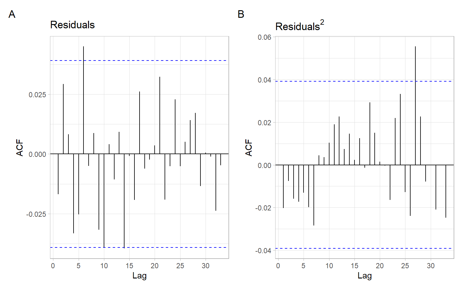
Next, we run diagnostics of the fitted model, i.e., whether the residuals \(\varepsilon_{t}\) are white noise and are normally distributed. The code plot(garch11) generates scatterplots, histograms, Q-Q plots, and ACF plots of the original data and the obtained residuals (Figure 6.4). Of course, the analysis can be performed also with separate commands. For example, see the ACFs of the residuals (Figure 6.5).

Code

par(mfrow = c(1, 2))
plot(garch11, which = c(3, 13))

Figure 6.4: Selected diagnostics of the GARCH(1,1) model for the USD/CAD log returns.

Code

et <- residuals(garch11, standardize = TRUE)
p1 <- forecast::ggAcf(et) +
    ggtitle("Residuals")
p2 <- forecast::ggAcf(et^2) +
    ggtitle(bquote('Residuals'^2))
p1 + p2 +
    plot_annotation(tag_levels = 'A')

Figure 6.5: ACF of residuals from the GARCH(1,1) model for the USD/CAD log returns.

Based on the plots, autocorrelations were effectively removed, but the assumption of normality is violated – Figure 6.4 shows heavy and almost symmetric tails in the distribution of GARCH residuals.

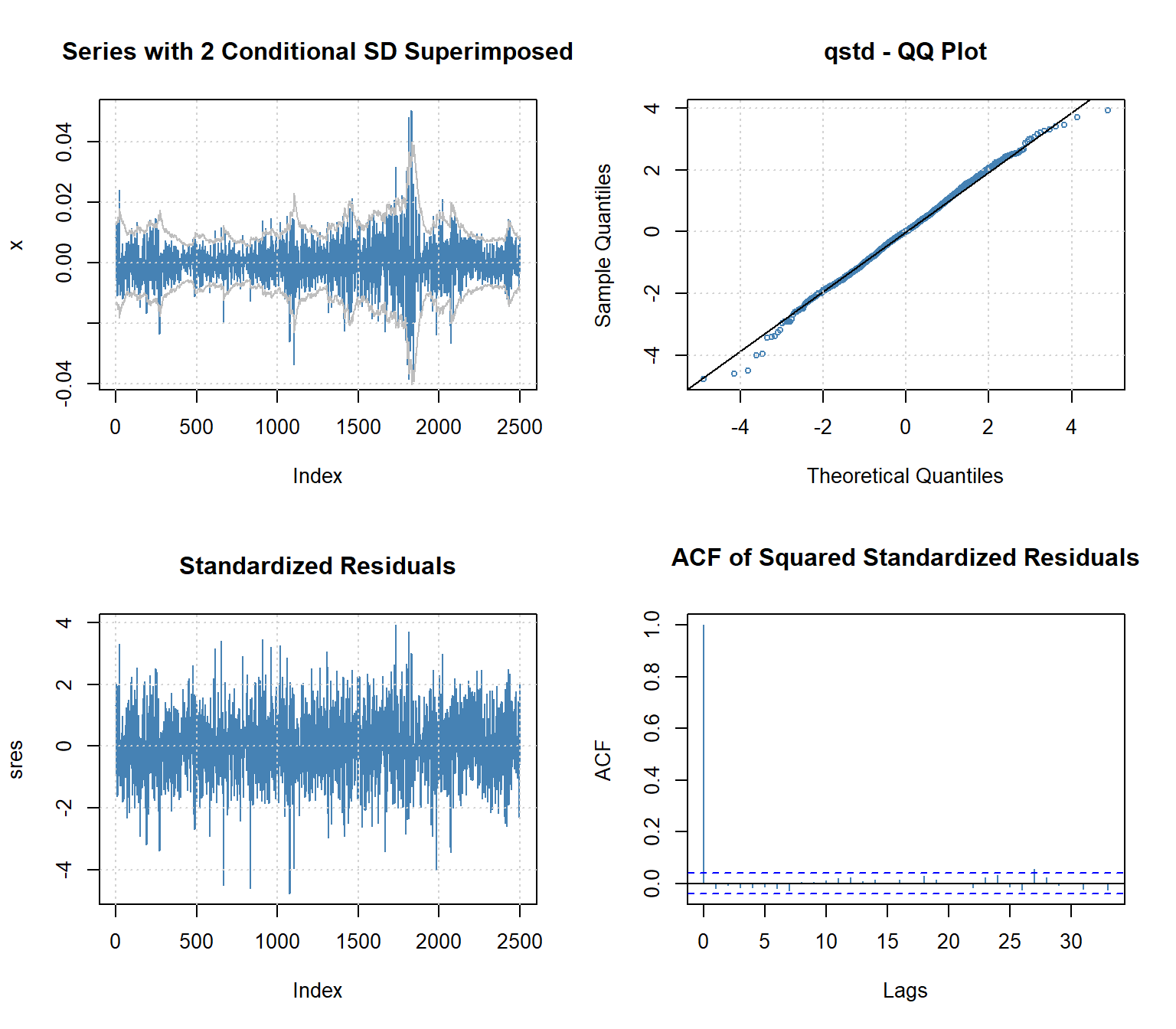
To account for the heavy tails, we change the conditional distribution from normal to the standardized Student \(t\)-distribution (see ?fGarch::std).

garch11t <- fGarch::garchFit(lnR ~ garch(1, 1),
                             data = CAD, trace = FALSE, 
                             cond.dist = "std")
garch11t@description <- "---"
garch11t

#> 
#> Title:
#>  GARCH Modelling 
#> 
#> Call:
#>  fGarch::garchFit(formula = lnR ~ garch(1, 1), data = CAD, cond.dist = "std", 
#>     trace = FALSE) 
#> 
#> Mean and Variance Equation:
#>  lnR ~ garch(1, 1)
#>  [data = CAD]
#> 
#> Conditional Distribution:
#>  std 
#> 
#> Coefficient(s):
#>          mu        omega       alpha1        beta1        shape  
#> -3.1972e-05   1.8744e-07   5.5352e-02   9.4057e-01   8.6423e+00  
#> 
#> Std. Errors:
#>  based on Hessian 
#> 
#> Error Analysis:
#>          Estimate  Std. Error  t value Pr(>|t|)    
#> mu     -3.197e-05   9.433e-05   -0.339   0.7346    
#> omega   1.874e-07   8.038e-08    2.332   0.0197 *  
#> alpha1  5.535e-02   7.765e-03    7.128 1.02e-12 ***
#> beta1   9.406e-01   7.760e-03  121.209  < 2e-16 ***
#> shape   8.642e+00   1.420e+00    6.084 1.17e-09 ***
#> ---
#> Signif. codes:  0 '***' 0.001 '**' 0.01 '*' 0.05 '.' 0.1 ' ' 1
#> 
#> Log Likelihood:
#>  9473    normalized:  3.78 
#> 
#> Description:
#>  ---

Verify the diagnostics plots in Figure 6.6.

Code

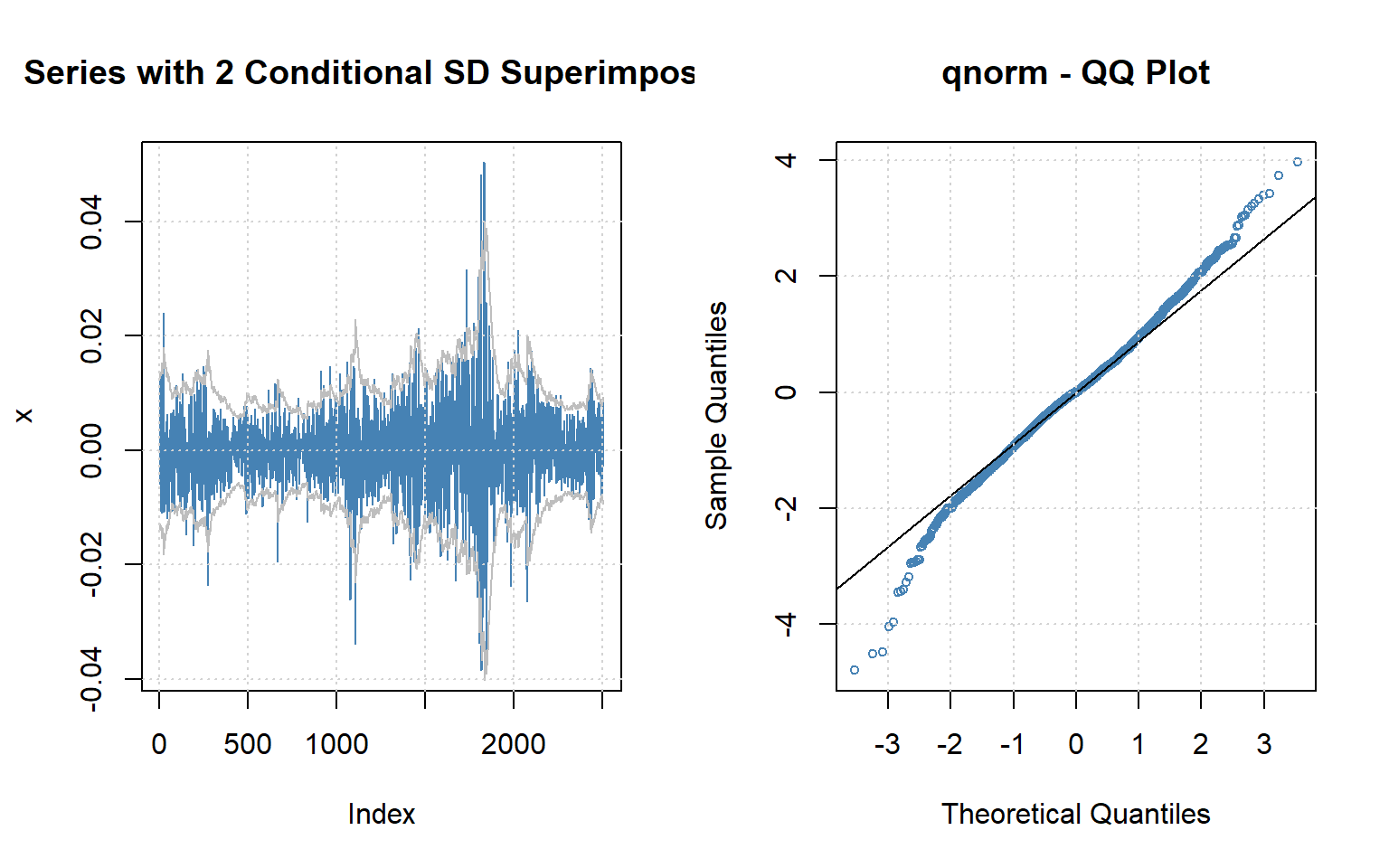
par(mfrow = c(2, 2))
plot(garch11t, which = c(3, 13))
plot(garch11t, which = c(9, 11))

Figure 6.6: Selected diagnostics of the GARCH(1,1) model with the standardized Student-t distribution for the USD/CAD log returns.

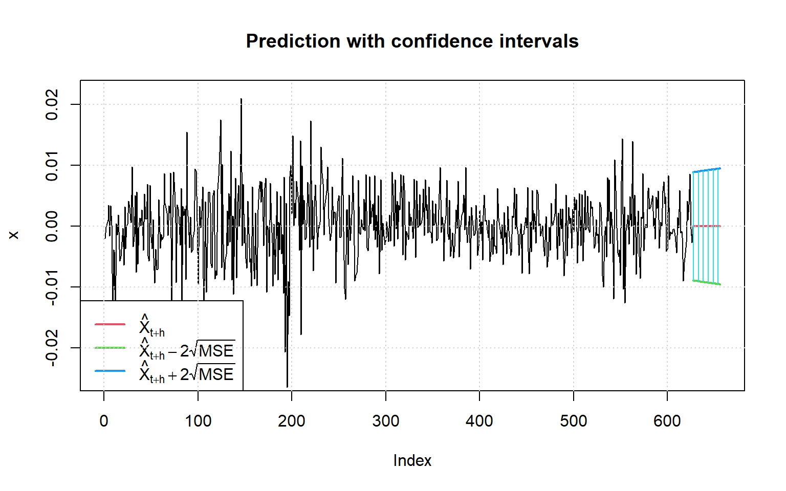
Now we can use the model for predictions (Figure 6.7). Few things to note here:

• the model is ‘self-contained’ so we can just specify n.ahead for the number of steps to be predicted;
• GARCH models are typically applied to long time series, so the argument nx limits the length of the plotted observed time series (by default only the most recent 25% of observations are plotted);
• the argument conf specifies the confidence level, then the conditional distribution from the model is used to compute critical values for the interval forecasts. Alternatively, one can specify the critical values manually with the argument crit_val.

For more details, see ?fGarch::predict.

Code

predict(garch11t, n.ahead = 30, 
        conf = 0.95,
        plot = TRUE)

#>    meanForecast meanError standardDeviation lowerInterval upperInterval
#> 1      -3.2e-05   0.00445           0.00445      -0.00892       0.00885
#> 2      -3.2e-05   0.00446           0.00446      -0.00894       0.00888
#> 3      -3.2e-05   0.00448           0.00448      -0.00896       0.00890
#> 4      -3.2e-05   0.00449           0.00449      -0.00899       0.00892
#> 5      -3.2e-05   0.00450           0.00450      -0.00901       0.00895
#> 6      -3.2e-05   0.00451           0.00451      -0.00903       0.00897
#> 7      -3.2e-05   0.00452           0.00452      -0.00906       0.00899
#> 8      -3.2e-05   0.00453           0.00453      -0.00908       0.00902
#> 9      -3.2e-05   0.00455           0.00455      -0.00910       0.00904
#> 10     -3.2e-05   0.00456           0.00456      -0.00913       0.00906
#> 11     -3.2e-05   0.00457           0.00457      -0.00915       0.00908
#> 12     -3.2e-05   0.00458           0.00458      -0.00917       0.00911
#> 13     -3.2e-05   0.00459           0.00459      -0.00919       0.00913
#> 14     -3.2e-05   0.00460           0.00460      -0.00921       0.00915
#> 15     -3.2e-05   0.00461           0.00461      -0.00924       0.00917
#> 16     -3.2e-05   0.00462           0.00462      -0.00926       0.00919
#> 17     -3.2e-05   0.00463           0.00463      -0.00928       0.00922
#> 18     -3.2e-05   0.00464           0.00464      -0.00930       0.00924
#> 19     -3.2e-05   0.00466           0.00466      -0.00932       0.00926
#> 20     -3.2e-05   0.00467           0.00467      -0.00934       0.00928
#> 21     -3.2e-05   0.00468           0.00468      -0.00937       0.00930
#> 22     -3.2e-05   0.00469           0.00469      -0.00939       0.00932
#> 23     -3.2e-05   0.00470           0.00470      -0.00941       0.00934
#> 24     -3.2e-05   0.00471           0.00471      -0.00943       0.00936
#> 25     -3.2e-05   0.00472           0.00472      -0.00945       0.00938
#> 26     -3.2e-05   0.00473           0.00473      -0.00947       0.00940
#> 27     -3.2e-05   0.00474           0.00474      -0.00949       0.00942
#> 28     -3.2e-05   0.00475           0.00475      -0.00951       0.00945
#> 29     -3.2e-05   0.00476           0.00476      -0.00953       0.00947
#> 30     -3.2e-05   0.00477           0.00477      -0.00955       0.00949

Figure 6.7: Predictions using the GARCH(1,1) model for the USD/CAD log returns.

6.4 Extensions

There was a boom in creating new models by adding new features to GARCH:

• IGARCH – integrated GARCH
• EGARCH – exponential GARCH
• TGARCH – threshold GARCH
• QGARCH – quadratic GARCH
• GARCH-M – GARCH with heteroskedasticity in mean
• NGARCH – nonlinear GARCH
• …
• MARCH – modified GARCH
• STARCH – structural ARCH
• …

Thus, these papers had to appear: Hansen and Lunde (2005) and Bollerslev (2009).

6.5 Model building

We have considered the models for conditional heteroskedasticity, and in the example, we estimated the mean just as a constant (intercept mu), however, in a more general case one might need to model and remove trend and cyclical variability along with autocorrelations (recall the methods of smoothing, ARMA, and ARIMA modeling) before exploring the need to model ARCH.

Below are the steps for such a more general case of analysis, adapted from Chapter 3.3 in Tsay (2005):

1. Specify a mean equation by testing for trend and serial dependence in the data and, if necessary, build a time series model (e.g., an ARMA model) to remove any linear dependence.
2. Use the residuals of the mean equation to test for ARCH effects.
3. If the ARCH effects are statistically significant, specify a volatility model and perform a joint estimation of the mean and volatility equations.
4. Check the fitted model carefully and refine it if necessary.

Note

The joint estimation can be done in R using the function fGarch::garchFit() and specifying, e.g., formula = ~ arma(2, 1) + garch(1, 1).

6.6 Conclusion

Whereas originated in financial analysis, GARCH models are becoming popular in other domains, including environmental science. Note that close alternatives exist, for example, GAMLSS allows modeling different distributional parameters such as mean, scale, skewness, etc.

GARCH effects are tested for and modeled after the mean (i.e., trend) and autocorrelations are removed. Standard model selection techniques can be adapted to specify GARCH models.

R packages offering functions for GARCH modeling include (in alphabetic order): bayesforecast, betategarch, fGarch (used here), garchx, rmgarch, rugarch, tseries, and more (see, for example, CRAN Task Views on Empirical Finance).

Bollerslev T (1986) Generalized autoregressive conditional heteroskedasticity. Journal of Econometrics 31:307–327. https://doi.org/10.1016/0304-4076(86)90063-1

Bollerslev T (2009) Glossary to ARCH (GARCH). In: Volatility and time series econometrics: Essays in honour of Robert F. Engle. SSRN

Brooks C, Burke SP (2003) Information criteria for GARCH model selection. The European Journal of Finance 9:557–580. https://doi.org/10.1080/1351847021000029188

Campbell SD, Diebold FX (2005) Weather forecasting for weather derivatives. Journal of the American Statistical Association 100:6–16. https://doi.org/10.1198/016214504000001051

Cripps E, Dunsmuir WTM (2003) Modeling the variability of Sydney Harbor wind measurements. Journal of Applied Meteorology 42:1131–1138. https://doi.org/10.1175/1520-0450(2003)042<1131:MTVOSH>2.0.CO;2

Engle RF (1982) Autoregressive conditional heteroscedasticity with estimates of the variance of United Kingdom inflation. Econometrica 50:987–1007. https://doi.org/10.2307/1912773

Hansen PR, Lunde A (2005) A comparison of volatility models: Does anything beat a GARCH(1, 1)? Journal of Applied Econometrics 20:873–889. https://doi.org/10.1002/jae.800

Kirchgässner G, Wolters J (2007) Introduction to modern time series analysis. Springer-Verlag, Berlin, Germany

Marinova D, McAleer M (2003) Modelling trends and volatility in ecological patents in the USA. Environmental Modelling & Software 18:195–203. https://doi.org/10.1016/S1364-8152(02)00079-8

Rydberg TH (2000) Realistic statistical modelling of financial data. International Statistical Review 68:233–258. https://doi.org/10.2307/1403412

Taylor JW, Buizza R (2004) A comparison of temperature density forecasts from GARCH and atmospheric models. Journal of Forecasting 23:337–355. https://doi.org/10.1002/for.917

Tsay RS (2005) Analysis of financial time series, 2nd edn. John Wiley & Sons, Hoboken, NJ, USA