Appendix C — Synchrony of parametric trends

The problem of detecting joint trend dynamics in time series is essential in a variety of applications, ranging from the analysis of macroeconomic indicators (Vogelsang and Franses 2005; Eun and Lee 2010) to assessing patterns in ice phenology measurements from multiple locations (Latifovic and Pouliot 2007; Duguay et al. 2013) to evaluating yields of financial instruments at various maturity levels (Park et al. 2009) and cell phone download activity at different area codes (Degras et al. 2012).

The extensive research on comparing trend patterns follows two main directions:

1. Testing for joint mean functions.
2. Analysis of joint stochastic trends, which is closely linked to the cointegration notion by Engle and Granger (1987) (Section 8.3).

Here we explore the first direction, that is, assess whether several observed time series follow the same hypothesized parametric trend.

There exist many tests for comparing mean functions, but most of the developed methods assume independent errors. Substantially less is known about testing for joint deterministic trends in a time series framework.

One of the methods developed for time series is by Degras et al. (2012) and Zhang (2013) who extended the integrated square error (ISE) based approach of Vilar-Fernández and González-Manteiga (2004) to a case of multiple time series with weakly dependent (non)stationary errors. For a comprehensive literature review of available methodology for comparing mean functions embedded into independent errors in a time series framework, see Degras et al. (2012) and Park et al. (2014). Most of these methods, however, either focus on aligning only two curves or require us to select multiple hyperparameters, such as the bandwidth, level of smoothness, and window size for a long-run variance function. As mentioned by Park et al. (2014), the choice of such multiple nuisance parameters is challenging for a comparison of curves (even under the independent and identically distributed setup) and often leads to inadequate performance, especially in samples of moderate size.

As an alternative, consider an extension of the WAVK test (Section 7.4.2) to a case of multiple time series (Lyubchich and Gel 2016). Let us observe \(N\) time series \[ Y_{it} = \mu_i(t/T) + \epsilon_{it}, \] where \(i = 1, \dots, N\) (\(N\) is the number of time series), \(t=1, \dots, T\) (\(T\) is the length of the time series), \(\mu_i(u)\) (\(0<u\leqslant 1\)) are unknown smooth trend functions, and the noise \(\epsilon_{it}\) can be represented as a finite-order AR(\(p\)) process or infinite-order AR(\(\infty\)) process with i.i.d. innovations \({e}_{it}\).

We are interested in testing whether these \(N\) observed time series have the same trend of some pre-specified smooth parametric form \(f(\theta, u)\):

\(H_0\): \(\mu_i(u)= c_i + f(\theta, u)\)
\(H_1\): there exists \(i\), such that \(\mu_i(u)\neq c_i + f(\theta, u)\),

where the reference curve \(f(\theta, u)\) with a vector of parameters \(\theta\) belongs to a known family of smooth parametric functions, and \(1\leqslant i \leqslant N\). For identifiability, assume that \(\sum_{i=1}^N c_i=0\). Notice that the hypotheses include (but are not limited to) the special cases of
\(f(\theta,u)\equiv 0\) (testing for no trend);
\(f(\theta,u)=\theta_0+\theta_1 u\) (testing for a common linear trend);
\(f(\theta,u)=\theta_0+\theta_1 u+\theta_2u^2\) (testing for a common quadratic trend).

This hypothesis testing approach allows us to answer the following questions:

• Do trends in temperature (or wind speeds, or precipitation) reproduced by a climate model correspond to the historical observations? I.e., is the model generally correct?
• Do different instruments (sensors) capture changes similarly, or deviate, for example, due to aging of some of the instruments?
• Do trends estimated at different locations (Canada and USA, lower and mid-troposphere, etc.) follow some hypothesized global trend?

Test the null hypothesis by following these steps (Lyubchich and Gel 2016):

1. Estimate the joint hypothetical trend \(f({\theta}, u)\) using the aggregated sample \(\left\{\overline{Y}_{\cdot t}\right\}_{t=1}^T\) (i.e., a time series obtained by averaging across all \(N\) time series).
2. For each time series, subtract the estimated trend, then apply the autoregressive filter to obtain residuals \(\hat{e}_{it}\), which under the \(H_0\) behave asymptotically like the independent and identically distributed \({e}_{it}\): \[ \begin{split} \hat{e}_{it}&= \hat{\epsilon}_{it}-\sum_{j=1}^{p_i(T)}{\hat{\phi}_{ij}\hat{\epsilon}_{i,t-j}} \\ &= \left\{ Y_{it} - f(\hat{\theta},u_{t}) \right\} - \left\{ \sum_{j=1}^{p_i(T)}{\hat{\phi}_{ij}{Y}_{i,t-j}} - \sum_{j=1}^{p_i(T)}{\hat{\phi}_{ij}f(\hat{\theta},u_{t-j})} \right\}. \end{split} \]
3. Construct a sequence of \(N\) statistics \({\rm WAVK}_{1}(k_{1}), \dots, {\rm WAVK}_{N}(k_{N})\). Then, the synchrony test statistic is \[ S_T = \sum_{i=1}^N k_{i}^{-1/2}{\rm WAVK}_{i}(k_{i}), \] where \(k_{i}\) is the local window size for the WAVK statistic.
4. Estimate the variance of \(\hat{e}_{it}\), e.g., using the robust difference-based estimator by Rice (1984): \[ s_i^2= \frac{\sum_{t=2}^T(\hat{e}_{it}-\hat{e}_{i,t-1})^2}{2(T-1)}. \]
5. Simulate \(BN\) times \(T\)-dimensional vectors \(e^*_{iT}\) from the multivariate normal distribution \(MVN\left(0, s_i^2\boldsymbol{I}\right)\), where \(B\) is the number of bootstrap replications, \(\boldsymbol{I}\) is a \(T\times T\) identity matrix.
6. Compute \(B\) bootstrapped statistics on \(e^*_{iT}\): \[S^*_T=\sum_{i=1}^N k^{-1/2}_{i} {\rm WAVK}^*_{i}(k_{i}).\]
7. The bootstrap \(p\)-value for testing the \(H_0\) is the proportion of \(|S^*_T|\) that exceed \(|S_T|\).

See the application of both the WAVK and synchrony tests in Lyubchich (2016).

If the null hypothesis is rejected, the method does not tell, however, what was the reason, and which particular time series caused the rejection of the \(H_0\). One can remove the time series (or several time series at once) with the largest WAVK statistic(s) and apply the test again, although repeated testing increases the probability of Type I error. For an application of this method in trend clustering, see this vignette.

Example: CMIP5 vs. observations

Replicate the test for synchrony of trends found in two time series (Lyubchich 2016):

• a multi-model average of temperatures from the 5th phase of the Coupled Model Intercomparison Project (CMIP5) and
• observed global temperature anomalies relative to the base period of 1981–2010.

Code

D <- read.csv("data/CMIP5.csv") %>% 
    filter(1948 <= Year & Year <= 2013) %>%
    mutate(Temp_CMIP5 = Temp_CMIP5 - 273.15)

See Figure C.1 showing the time series plots after converting the CMIP data to degrees Celsius.

Code

p1 <- D %>% ggplot(aes(x = Year, y = Temp_CMIP5)) +
    geom_line()
p2 <- D %>% ggplot(aes(x = Year, y = Temp_obs)) +
    geom_line()
p1 + p2 +
    plot_annotation(tag_levels = 'A')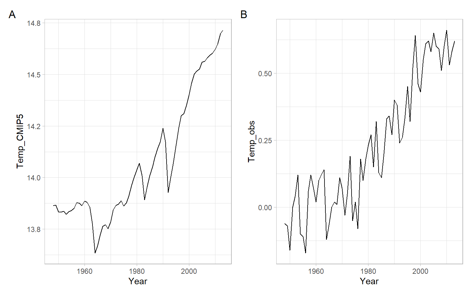

Figure C.1: Global annual mean temperature (°C) in 1948–2013: CMIP5 multi-model average and observed anomalies relative to the base period of 1981–2010.

Test the synchrony of parametric linear trends in these time series:

set.seed(123)
funtimes::sync_test(D[, c("Temp_CMIP5", "Temp_obs")] ~ t)

#> 
#>  Nonparametric test for synchronism of parametric trends
#> 
#> data:  D[, c("Temp_CMIP5", "Temp_obs")] 
#> Test statistic = 0.04, p-value = 0.03
#> alternative hypothesis: common trend is not of the form D[, c("Temp_CMIP5", "Temp_obs")] ~ t.
#> sample estimates:
#> $common_trend_estimates
#>             Estimate Std. Error t value Pr(>|t|)
#> (Intercept)    -1.57     0.0962   -16.4 1.44e-24
#> t               3.10     0.1647    18.8 8.39e-28
#> 
#> $ar.order_used
#>          Temp_CMIP5 Temp_obs
#> ar.order          1        1
#> 
#> $Window_used
#>        Temp_CMIP5 Temp_obs
#> Window          3        3
#> 
#> $all_considered_windows
#>  Window Statistic p-value Asympt. p-value
#>       3    0.0406   0.034          0.0246
#>       4    0.0373   0.042          0.0386
#>       6    0.0413   0.020          0.0222
#> 
#> $wavk_obs
#> [1] 0.0143 0.0263

The \(p\)-value below the usual significance level \(\alpha = 0.05\) allows us to reject the null hypothesis, however, as Lyubchich (2016) pointed out, the decision would differ if more confidence is required (e.g., \(\alpha = 0.01\)). Note that the \(p\)-value of 0.012 reported by Lyubchich (2016) differs from the one reported above due to the function settings and randomness due to the bootstrapping. We should save the random number generator state with set.seed() for replicability (so the test results are exactly the same every time the test is applied), and use a larger number of bootstrap replications B for consistency (so the test leads to the same conclusions when the function set.seed() is not used).

Now test the synchrony of parametric quadratic trends in these time series:

set.seed(123)
funtimes::sync_test(D[, c("Temp_CMIP5", "Temp_obs")] ~ poly(t, 2))

#> 
#>  Nonparametric test for synchronism of parametric trends
#> 
#> data:  D[, c("Temp_CMIP5", "Temp_obs")] 
#> Test statistic = 0.05, p-value = 0.002
#> alternative hypothesis: common trend is not of the form D[, c("Temp_CMIP5", "Temp_obs")] ~ poly(t, 2).
#> sample estimates:
#> $common_trend_estimates
#>             Estimate Std. Error  t value Pr(>|t|)
#> (Intercept) 7.52e-16     0.0324 2.32e-14 1.00e+00
#> poly(t, 2)1 7.27e+00     0.2632 2.76e+01 6.20e-37
#> poly(t, 2)2 2.28e+00     0.2632 8.65e+00 2.62e-12
#> 
#> $ar.order_used
#>          Temp_CMIP5 Temp_obs
#> ar.order          2        0
#> 
#> $Window_used
#>        Temp_CMIP5 Temp_obs
#> Window          3        3
#> 
#> $all_considered_windows
#>  Window Statistic p-value Asympt. p-value
#>       3    0.0518   0.002        0.000282
#>       4    0.0350   0.028        0.014236
#>       6    0.0222   0.070        0.120094
#> 
#> $wavk_obs
#> [1] -0.000673  0.052504

Note these results differ substantially based on the window used for computing the WAVK statistic. The function funtimes::sync_test() automatically selects the optimal window based on the heuristic approach of comparing distances between bootstrap distributions (Lyubchich 2016; Lyubchich and Gel 2016).

Degras D, Xu Z, Zhang T, Wu WB (2012) Testing for parallelism among trends in multiple time series. IEEE Transactions on Signal Processing 60:1087–1097. https://doi.org/10.1109/TSP.2011.2177831

Duguay CR, Brown L, Kang K-K, Kheyrollah Pour H (2013) State of the climate in 2012: Lake ice. Bulletin of the American Meteorological Society 94:S124–S126. https://doi.org/10.1175/2013BAMSStateoftheClimate.1

Engle RF, Granger CWJ (1987) Co-integration and error correction: Representation, estimation, and testing. Econometrica 55:251–276. https://doi.org/10.2307/1913236

Eun CS, Lee J (2010) Mean-variance convergence around the world. Journal of Banking & Finance 34:856–870. https://doi.org/10.1016/j.jbankfin.2009.09.016

Latifovic R, Pouliot D (2007) Analysis of climate change impacts on lake ice phenology in Canada using the historical satellite data record. Remote Sensing of Environment 106:492–507. https://doi.org/10.1016/j.rse.2006.09.015

Lyubchich V (2016) Detecting time series trends and their synchronization in climate data. Intelligence Innovations Investments 12:132–137. https://www.researchgate.net/publication/318283780_Detecting_time_series_trends_and_their_synchronization_in_climate_data

Lyubchich V, Gel YR (2016) A local factor nonparametric test for trend synchronism in multiple time series. Journal of Multivariate Analysis 150:91–104. https://doi.org/10.1016/j.jmva.2016.05.004

Park C, Hannig J, Kang K-H (2014) Nonparametric comparison of multiple regression curves in scale-space. Journal of Computational and Graphical Statistics 23:657–677. https://doi.org/10.1080/10618600.2013.822816

Park C, Vaughan A, Hannig J, Kang K-H (2009) SiZer analysis for the comparison of time series. Journal of Statistical Planning and Inference 139:3974–3988. https://doi.org/10.1016/j.jspi.2009.05.003

Rice J (1984) Bandwidth choice for nonparametric regression. The Annals of Statistics 12:1215–1230. https://doi.org/10.1214/aos/1176346788

Vilar-Fernández JM, González-Manteiga W (2004) Nonparametric comparison of curves with dependent errors. Statistics 38:81–99. https://doi.org/10.1080/02331880310001634656

Vogelsang TJ, Franses PH (2005) Testing for common deterministic trend slopes. Journal of Econometrics 126:1–24. https://doi.org/10.1016/j.jeconom.2004.02.004

Zhang T (2013) Clustering high-dimensional time series based on parallelism. Journal of the American Statistical Association 108:577–588. https://doi.org/10.1080/01621459.2012.760458