Appendix B — Generalized least squares

Here we use time series data (ordered by \(t\)), thus, Equation A.1 will be written with the time indices \(t\) as \[ y_t=\beta_0+\beta_1x_t+\varepsilon_t, \tag{B.1}\] where the regression errors at times \(t\) and \(t-1\) are \[ \begin{split} \varepsilon_t&=y_t-\beta_0-\beta_1x_t,\\ \varepsilon_{t-1}&=y_{t-1}-\beta_0-\beta_1x_{t-1}. \end{split} \tag{B.2}\]

An AR(1) model for the errors will yield \[ \begin{split} y_t-\beta_0-\beta_1x_t & = \rho\varepsilon_{t-1} + w_t, \\ y_t-\beta_0-\beta_1x_t & = \rho(y_{t-1}-\beta_0-\beta_1x_{t-1})+w_t, \end{split} \tag{B.3}\] where \(w_t\) are uncorrelated errors.

Rewrite it as \[ \begin{split} y_t-\rho y_{t-1}&=\beta_0(1-\rho)+\beta_1(x_t-\rho x_{t-1})+w_t,\\ y_t^* &= \beta_0^* + \beta_1 x_t^*+w_t, \end{split} \tag{B.4}\] where \(y_t^* = y_t-\rho y_{t-1}\); \(\beta_0^* = \beta_0(1-\rho)\); \(x_t^* = x_t-\rho x_{t-1}\). Notice the errors \(w_t\) in the final Equation B.4 for the transformed variables \(y_t^*\) and \(x_t^*\) are uncorrelated.

To get from Equation B.1 to Equation B.4, we can use an iterative procedure by Cochrane and Orcutt (1949) as in the example below.

Example: Dishwasher shipments model accounting for autocorrelation

1. Estimate the model in Equation B.1 using OLS.

Code

D <- read.delim("data/dish.txt") %>% 
    rename(Year = YEAR)
modDish_ols <- lm(DISH ~ RES, data = D)

2. Calculate residuals \(\hat{\varepsilon}_t\) and estimate \(\rho\) as \[ \hat{\rho}=\frac{\sum_{t=2}^n\hat{\varepsilon}_t\hat{\varepsilon}_{t-1}}{\sum_{t=1}^n\hat{\varepsilon}^2_t}. \]

Code

e <- modDish_ols$residuals
rho <- sum(e[-1] * e[-length(e)]) / sum(e^2)
rho

#> [1] 0.694

3. Calculate transformed variables \(x^*_t\) and \(y^*_t\) and fit model in Equation B.4.

Code

y.star <- D$DISH[-1] - rho * D$DISH[-length(D$DISH)]
x.star <- D$RES[-1] - rho * D$RES[-length(D$RES)]
modDish_ar1 <- lm(y.star ~ x.star)
summary(modDish_ar1)

#> 
#> Call:
#> lm(formula = y.star ~ x.star)
#> 
#> Residuals:
#>    Min     1Q Median     3Q    Max 
#> -479.7 -117.8   32.9  120.7  536.1 
#> 
#> Coefficients:
#>             Estimate Std. Error t value Pr(>|t|)    
#> (Intercept)    26.76     130.69    0.20     0.84    
#> x.star         50.99       7.74    6.59    1e-06 ***
#> ---
#> Signif. codes:  0 '***' 0.001 '**' 0.01 '*' 0.05 '.' 0.1 ' ' 1
#> 
#> Residual standard error: 252 on 23 degrees of freedom
#> Multiple R-squared:  0.654,  Adjusted R-squared:  0.639 
#> F-statistic: 43.4 on 1 and 23 DF,  p-value: 1.01e-06

4. Examine the residuals of the newly fitted equation (Figure B.1) and repeat the procedure, if needed.

Code

p1 <- ggplot(D, aes(x = Year, y = modDish_ols$residuals)) + 
    geom_line() + 
    geom_hline(yintercept = 0, lty = 2, col = 4) + 
    ggtitle("OLS model modDish_ols") +
    ylab("Residuals")
p2 <- ggplot(D[-1,], aes(x = Year, y = modDish_ar1$residuals)) + 
    geom_line() + 
    geom_hline(yintercept = 0, lty = 2, col = 4) + 
    ggtitle("Transformed model modDish_ar1") +
    ylab("Residuals")
p1 + p2 +
    plot_annotation(tag_levels = 'A')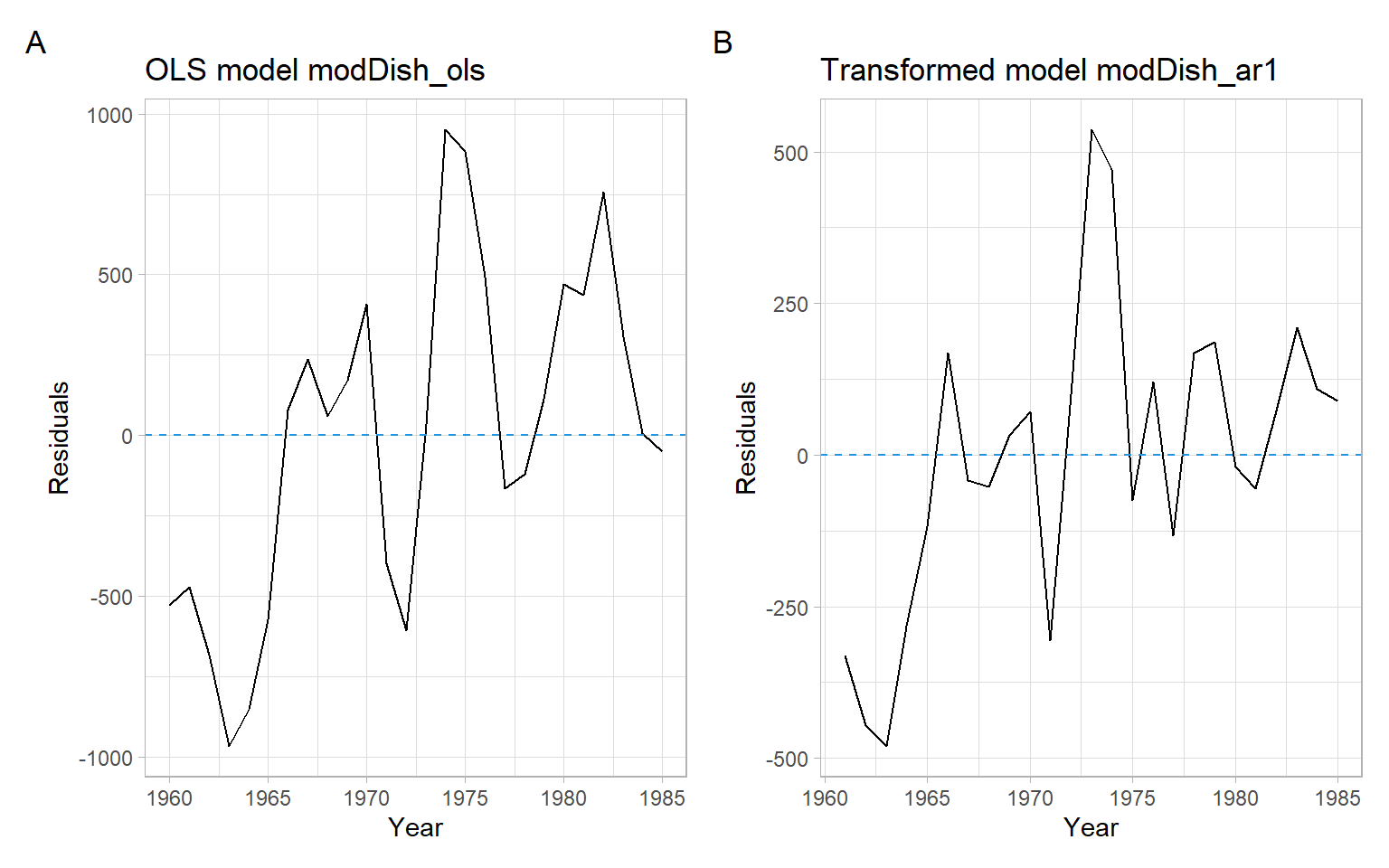

Figure B.1: Residual plots of the original OLS model and the model transformed to account for autocorrelation in residuals.

Based on the runs test, there is not enough evidence of autocorrelation in the new residuals:

lawstat::runs.test(rstandard(modDish_ar1))

#> 
#>  Runs Test - Two sided
#> 
#> data:  rstandard(modDish_ar1)
#> Standardized Runs Statistic = -0.6, p-value = 0.5

What we have just applied is the method of generalized least squares (GLS): \[ \hat{\boldsymbol{\beta}} = \left( \boldsymbol{X}^{\top}\boldsymbol{\Sigma}^{-1}\boldsymbol{X}\right)^{-1} \boldsymbol{X}^{\top}\boldsymbol{\Sigma}^{-1}\boldsymbol{Y}, \tag{B.5}\] where \(\boldsymbol{\Sigma}\) is the covariance matrix. The method of weighted least squares (WLS; Appendix A) is just a special case of the GLS. In the WLS approach, all the off-diagonal entries of \(\boldsymbol{\Sigma}\) are 0.

We can use the function nlme::gls() and specify the correlation structure to avoid iterating the steps from the previous example manually:

modDish_ar1_v2 <- nlme::gls(DISH ~ RES
                            ,correlation = nlme::corAR1(form = ~Year)
                            ,data = D)
summary(modDish_ar1_v2)

#> Generalized least squares fit by REML
#>   Model: DISH ~ RES 
#>   Data: D 
#>   AIC BIC logLik
#>   342 347   -167
#> 
#> Correlation Structure: AR(1)
#>  Formula: ~Year 
#>  Parameter estimate(s):
#> Phi 
#>   1 
#> 
#> Coefficients:
#>              Value Std.Error t-value p-value
#> (Intercept) -137.5   3714137    0.00       1
#> RES           45.7         6    7.35       0
#> 
#>  Correlation: 
#>     (Intr)
#> RES 0     
#> 
#> Standardized residuals:
#>       Min        Q1       Med        Q3       Max 
#> -0.000249 -0.000014  0.000135  0.000232  0.000338 
#> 
#> Residual standard error: 3714137 
#> Degrees of freedom: 26 total; 24 residual

Note

In the function nlme::gls() we can also specify weights to accommodate heteroskedastic errors, but the syntax differs from the weights specification in the function stats::lm() (Appendix A). See ?nlme::varFixed.

Cochrane D, Orcutt GH (1949) Application of least squares regression to relationships containing auto-correlated error terms. Journal of the American Statistical Association 44:32–61. https://doi.org/10.2307/2280349